-
 Ross Ihaka
 -
 Robert Gentleman
R (programming language) Source: en.wikipedia.org/wiki/R_(programming_language)
| R | |
|---|---|
 Terminal window for R | |
| Paradigms | Multi-paradigm: procedural, object-oriented, functional, reflective, imperative, array[1] |
| Designed by | Ross Ihaka and Robert Gentleman |
| Developer | R Core Team |
| First appeared | August 1993 |
| Stable release | 4.5.1[2] |
| Typing discipline | Dynamic |
| Platform | arm64 and x86-64 |
| License | GPL-2.0-or-later[3] |
| Filename extensions | |
| Website | r-project.org |
| Influenced by | |
| Influenced | |
| Julia[7] pandas[8] | |
| |
R is a programming language for statistical computing and data visualization. It has been widely adopted in the fields of data mining, bioinformatics, data analysis, and data science.[9]
The core R language is extended by a large number of software packages, which contain reusable code, documentation, and sample data. Some of the most popular R packages are in the tidyverse collection, which enhances functionality for visualizing, transforming, and modelling data, as well as improves the ease of programming (according to the authors and users).[10]
R is free and open-source software distributed under the GNU General Public License.[3][11] The language is implemented primarily in C, Fortran, and R itself. Precompiled executables are available for the major operating systems (including Linux, MacOS, and Microsoft Windows).
Its core is an interpreted language with a native command line interface. In addition, multiple third-party applications are available as graphical user interfaces; such applications include RStudio (an integrated development environment) and Jupyter (a notebook interface).
History
[edit]Co-originators of the R language
.jpg)

R was started by professors Ross Ihaka and Robert Gentleman as a programming language to teach introductory statistics at the University of Auckland.[12] The language was inspired by the S programming language, with most S programs able to run unaltered in R.[6] The language was also inspired by Scheme's lexical scoping, allowing for local variables.[1]
The name of the language, R, comes from being both an S language successor and the shared first letter of the authors, Ross and Robert.[13] In August 1993, Ihaka and Gentleman posted a binary file of R on StatLib — a data archive website.[14] At the same time, they announced the posting on the s-news mailing list.[15] On 5 December 1997, R became a GNU project when version 0.60 was released.[16] On 29 February 2000, the 1.0 version was released.[17]
Packages
[edit]
R packages are collections of functions, documentation, and data that expand R.[18] For example, packages can add reporting features (using packages such as RMarkdown, Quarto,[19] knitr, and Sweave) and support for various statistical techniques (such as linear, generalized linear and nonlinear modeling, classical statistical tests, spatial analysis, time-series analysis, and clustering). Ease of package installation and use have contributed to the language's adoption in data science.[20]
Immediately available when starting R after installation, base packages provide the fundamental and necessary syntax and commands for programming, computing, graphics production, basic arithmetic, and statistical functionality.[21]
An example is the tidyverse collection of R packages, which bundles several subsidiary packages to provide a common API. The collection specializes in tasks related to accessing and processing "tidy data",[22] which are data contained in a two-dimensional table with a single row for each observation and a single column for each variable.[23]
Installing a package occurs only once. For example, to install the tidyverse collection:[23]
> install.packages("tidyverse")
To load the functions, data, and documentation of a package, one calls the library() function. To load the tidyverse collection, one can execute the following code:[a]
> # The package name can be enclosed in quotes
> library("tidyverse")

> # But the package name can also be used without quotes
> library(tidyverse)
The Comprehensive R Archive Network (CRAN) was founded in 1997 by Kurt Hornik and Friedrich Leisch to host R's source code, executable files, documentation, and user-created packages.[24] CRAN's name and scope mimic the Comprehensive TeX Archive Network (CTAN) and the Comprehensive Perl Archive Network (CPAN).[24] CRAN originally had only three mirror sites and twelve contributed packages.[25] As of 16 October 2024[update], it has 99 mirrors[26] and 21,513 contributed packages.[27] Packages are also available in repositories such as R-Forge, Omegahat, and GitHub.[28][29][30]
To provide guidance on the CRAN web site, its Task Views area lists packages that are relevant for specific topics; sample topics include causal inference, finance, genetics, high-performance computing, machine learning, medical imaging, meta-analysis, social sciences, and spatial statistics.
The Bioconductor project provides packages for genomic data analysis, complementary DNA, microarray, and high-throughput sequencing methods.
Community
[edit]There are three main groups that help support R software development:
- The R Core Team was founded in 1997 to maintain the R source code.
- The R Foundation for Statistical Computing was founded in April 2003 to provide financial support.
- The R Consortium is a Linux Foundation project to develop R infrastructure.
The R Journal is an open access, academic journal that features short to medium-length articles on the use and development of R. The journal includes articles on packages, programming tips, CRAN news, and foundation news.
The R community hosts many conferences and in-person meetups.[b] These groups include:
- UseR!: an annual international R user conference (website)
- Directions in Statistical Computing (DSC) (website)
- R-Ladies: an organization to promote gender diversity in the R community (website)
- SatRdays: R-focused conferences held on Saturdays (website)
- R Conference (website)
- posit::conf (formerly known as rstudio::conf) (website)
On social media sites such as Twitter, the hashtag #rstats can be used to follow new developments in the R community.[31]
Examples
[edit]Hello, World!
[edit]The following is a "Hello, World!" program:
> print("Hello, World!")
[1] "Hello, World!"
Here is an alternative version, which uses the cat() function:
> cat("Hello, World!")
Hello, World!
Basic syntax
[edit]The following examples illustrate the basic syntax of the language and use of the command-line interface.[c]
In R, the generally preferred assignment operator is an arrow made from two characters <-, although = can be used in some cases.[32]
> x <- 1:6 # Create a numeric vector in the current environment
> y <- x^2 # Similarly, create a vector based on the values in x.
> print(y) # Print the vector’s contents.
[1]  1  4  9 16 25 36

> z <- x + y # Create a new vector that is the sum of x and y
> z # Return the contents of z to the current environment.
[1]  2  6 12 20 30 42

> z_matrix <- matrix(z, nrow = 3) # Create a new matrix that transforms the vector z into a 3x2 matrix object
> z_matrix
     [,1] [,2]
[1,]    2   20
[2,]    6   30
[3,]   12   42

> 2 * t(z_matrix) - 2 # Transpose the matrix; multiply every element by 2; subtract 2 from each element in the matrix; and then return the results to the terminal.
     [,1] [,2] [,3]
[1,]    2   10   22
[2,]   38   58   82

> new_df <- data.frame(t(z_matrix), row.names = c("A", "B")) # Create a new dataframe object that contains the data from a transposed z_matrix, with row names 'A' and 'B'
> names(new_df) <- c("X", "Y", "Z") # Set the column names of the new_df dataframe as X, Y, and Z.
> print(new_df)  # Print the current results.
   X  Y  Z
A  2  6 12
B 20 30 42

> new_df$Z # Output the Z column
[1] 12 42

> new_df$Z == new_df['Z'] && new_df[3] == new_df$Z # The dataframe column Z can be accessed using the syntax $Z, ['Z'], or [3], and the values are the same.
[1] TRUE

> attributes(new_df) # Print information about attributes of the new_df dataframe
$names
[1] "X" "Y" "Z"

$row.names
[1] "A" "B"

$class
[1] "data.frame"

> attributes(new_df)$row.names <- c("one", "two") # Access and then change the row.names attribute; this can also be done using the rownames() function
> new_df
     X  Y  Z
one  2  6 12
two 20 30 42
Structure of a function
[edit]R is able to create functions that add new functionality for code reuse.[33] Objects created within the body of the function (which are enclosed by curly brackets) remain accessible only from within the function, and any data type may be returned. In R, almost all functions and all user-defined functions are closures.[34]
The following is an example of creating a function to perform an arithmetic calculation:
# The function's input parameters are x and y.
# The function, named f, returns a linear combination of x and y.
f <- function(x, y) {
  z <- 3 * x + 4 * y

  # An explicit return() statement is optional--it could be replaced with simply `z` in this case.
  return(z)
}

# As an alternative, the last statement executed in a function is returned implicitly.
f <- function(x, y) 3 * x + 4 * y
The following is some output from using the function defined above:
> f(1, 2) #  3 * 1 + 4 * 2 = 3 + 8
[1] 11

> f(c(1, 2, 3), c(5, 3, 4)) # Element-wise calculation
[1] 23 18 25

> f(1:3, 4) # Equivalent to f(c(1, 2, 3), c(4, 4, 4))
[1] 19 22 25
It is possible to define functions to be used as infix operators by using the special syntax `%name%`, where "name" is the function variable name:
> `%sumx2y2%` <- function(e1, e2) {e1 ^ 2 + e2 ^ 2}
> 1:3 %sumx2y2% -(1:3)
[1]  2  8 18
Since R version 4.1.0, functions can be written in a short notation, which is useful for passing anonymous functions to higher-order functions:[35]
> sapply(1:5, \(i) i^2)    # here \(i) is the same as function(i)
[1]  1  4  9 16 25
Native pipe operator
[edit]In R version 4.1.0, a native pipe operator, |>, was introduced.[36] This operator allows users to chain functions together, rather than using nested function calls.
> nrow(subset(mtcars, cyl == 4)) # Nested without the pipe character
[1] 11

> mtcars |> subset(cyl == 4) |> nrow() # Using the pipe character
[1] 11
Another alternative to nested functions is the use of intermediate objects, rather than the pipe operator:
> mtcars_subset_rows <- subset(mtcars, cyl == 4)
> num_mtcars_subset <- nrow(mtcars_subset_rows)
> print(num_mtcars_subset)
[1] 11
While the pipe operator can produce code that is easier to read, it is advisable to chain together at most 10-15 lines of code using this operator, as well as to chunk code into sub-tasks that are saved into objects having meaningful names.[37] The following is an example having fewer than 10 lines, which some readers may find difficult to grasp in the absence of intermediate named steps:
(\(x, n = 42, key = c(letters, LETTERS, " ", ":", ")"))
    strsplit(x, "")[[1]] |>
    (Vectorize(\(chr) which(chr == key) - 1))() |>
    (`+`)(n) |>
    (`%%`)(length(key)) |>
    (\(i) key[i + 1])() |>
    paste(collapse = "")
)("duvFkvFksnvEyLkHAErnqnoyr")
The following is a version of the preceding code that is easier to read:
default_key <- c(letters, LETTERS, " ", ":", ")")

f <- function(x, n = 42, key = default_key) {
    split_input <- strsplit(x, "")[[1]]
    results <- (Vectorize(\(chr) which(chr == key) - 1))(split_input) |>
        (`+`)(n) |>
        (`%%`)(length(key)) |>
        (\(i) key[i + 1])()
    combined_results <- paste(results, collapse = "")
    return(combined_results)
}

f("duvFkvFksnvEyLkHAErnqnoyr")
Object-oriented programming
[edit]The R language has native support for object-oriented programming. There are two native frameworks, the so-called S3 and S4 systems. The former, being more informal, supports single dispatch on the first argument, and objects are assigned to a class simply by setting a "class" attribute in each object. The latter is a system like the Common Lisp Object System (CLOS), with formal classes (also derived from S) and generic methods, which supports multiple dispatch and multiple inheritance[38]
In the example below, summary() is a generic function that dispatches to different methods depending on whether its argument is a numeric vector or a factor:
> data <- c("a", "b", "c", "a", NA)
> summary(data)
   Length     Class      Mode
        5 character character
> summary(as.factor(data))
   a    b    c NA's
   2    1    1    1
Modeling and plotting
[edit]
plot.lm() function). Mathematical notation is allowed in labels, as shown in the lower left plot.The R language has built-in support for data modeling and graphics. The following example shows how R can generate and plot a linear model with residuals.
# Create x and y values
x <- 1:6
y <- x^2

# Linear regression model: y = A + B * x
model <- lm(y ~ x)

# Display an in-depth summary of the model
summary(model)

# Create a 2-by-2 layout for figures
par(mfrow = c(2, 2))

# Output diagnostic plots of the model
plot(model)
The output from the summary() function in the preceding code block is as follows:
Residuals:
      1       2       3       4       5       6       7       8      9      10
 3.3333 -0.6667 -2.6667 -2.6667 -0.6667  3.3333

Coefficients:
            Estimate Std. Error t value Pr(>|t|)
(Intercept)  -9.3333     2.8441  -3.282 0.030453 *
x             7.0000     0.7303   9.585 0.000662 ***
---
Signif. codes:  0 ‘***’ 0.001 ‘**’ 0.01 ‘*’ 0.05 ‘.’ 0.1 ‘ ’ 1

Residual standard error: 3.055 on 4 degrees of freedom
Multiple R-squared:  0.9583, Adjusted R-squared:  0.9478
F-statistic: 91.88 on 1 and 4 DF,  p-value: 0.000662
Mandelbrot set
[edit]
This example of a Mandelbrot set highlights the use of complex numbers. It models the first 20 iterations of the equation z = z2 + c, where c represents different complex constants.
To run this sample code, it is necessary to first install the package that provides the write.gif() function:
install.packages("caTools")
The sample code is as follows:
library(caTools)

jet.colors <-
    colorRampPalette(
        c("green", "pink", "#007FFF", "cyan", "#7FFF7F",
          "white", "#FF7F00", "red", "#7F0000"))

dx <- 1500 # define width
dy <- 1400 # define height

C  <-
    complex(
            real = rep(seq(-2.2, 1.0, length.out = dx), each = dy),
            imag = rep(seq(-1.2, 1.2, length.out = dy), times = dx)
            )

# reshape as matrix of complex numbers
C <- matrix(C, dy, dx)

# initialize output 3D array
X <- array(0, c(dy, dx, 20))

Z <- 0

# loop with 20 iterations
for (k in 1:20) {

  # the central difference equation
  Z <- Z^2 + C

  # capture the results
  X[, , k] <- exp(-abs(Z))
}

write.gif(
    X,
    "Mandelbrot.gif",
    col = jet.colors,
    delay = 100)
Version names
[edit]
All R version releases from 2.14.0 onward have codenames that make reference to Peanuts comics and films.[39][40][41]
In 2018, core R developer Peter Dalgaard presented a history of R releases since 1997.[42] Some notable early releases before the named releases include the following:
- Version 1.0.0, released on 29 February 2000, a leap day
- Version 2.0.0, released on 4 October 2004, "which at least had a nice ring to it"[42]
The idea of naming R version releases was inspired by the naming system for Debian and Ubuntu versions. Dalgaard noted an additional reason for the use of Peanuts references in R codenames—the humorous observation that "everyone in statistics is a P-nut."[42]
| Version | Release date | Name | Peanuts reference | Reference |
|---|---|---|---|---|
| 4.5.1 | 2025-06-13 | Great Square Root | [43] | [44] |
| 4.5.0 | 2025-04-11 | How About a Twenty-Six | [45] | [46] |
| 4.4.3 | 2025-02-28 | Trophy Case | [47] | [48] |
| 4.4.2 | 2024-10-31 | Pile of Leaves | [49] | [50] |
| 4.4.1 | 2024-06-14 | Race for Your Life | [51] | [52] |
| 4.4.0 | 2024-04-24 | Puppy Cup | [53] | [54] |
| 4.3.3 | 2024-02-29 | Angel Food Cake | [55] | [56] |
| 4.3.2 | 2023-10-31 | Eye Holes | [57] | [58] |
| 4.3.1 | 2023-06-16 | Beagle Scouts | [59] | [60] |
| 4.3.0 | 2023-04-21 | Already Tomorrow | [61][62][63] | [64] |
| 4.2.3 | 2023-03-15 | Shortstop Beagle | [65] | [66] |
| 4.2.2 | 2022-10-31 | Innocent and Trusting | [67] | [68] |
| 4.2.1 | 2022-06-23 | Funny-Looking Kid | [69][70][71][72][73][74] | [75] |
| 4.2.0 | 2022-04-22 | Vigorous Calisthenics | [76] | [77] |
| 4.1.3 | 2022-03-10 | One Push-Up | [76] | [78] |
| 4.1.2 | 2021-11-01 | Bird Hippie | [79][80] | [78] |
| 4.1.1 | 2021-08-10 | Kick Things | [81] | [82] |
| 4.1.0 | 2021-05-18 | Camp Pontanezen | [83] | [84] |
| 4.0.5 | 2021-03-31 | Shake and Throw | [85] | [86] |
| 4.0.4 | 2021-02-15 | Lost Library Book | [87][88][89] | [90] |
| 4.0.3 | 2020-10-10 | Bunny-Wunnies Freak Out | [91] | [92] |
| 4.0.2 | 2020-06-22 | Taking Off Again | [93] | [94] |
| 4.0.1 | 2020-06-06 | See Things Now | [95] | [96] |
| 4.0.0 | 2020-04-24 | Arbor Day | [97] | [98] |
| 3.6.3 | 2020-02-29 | Holding the Windsock | [99] | [100] |
| 3.6.2 | 2019-12-12 | Dark and Stormy Night | See It was a dark and stormy night#Literature[101] | [102] |
| 3.6.1 | 2019-07-05 | Action of the Toes | [103] | [104] |
| 3.6.0 | 2019-04-26 | Planting of a Tree | [105] | [106] |
| 3.5.3 | 2019-03-11 | Great Truth | [107] | [108] |
| 3.5.2 | 2018-12-20 | Eggshell Igloos | [109] | [110] |
| 3.5.1 | 2018-07-02 | Feather Spray | [111] | [112] |
| 3.5.0 | 2018-04-23 | Joy in Playing | [113] | [114] |
| 3.4.4 | 2018-03-15 | Someone to Lean On | [115][116][117] | [118] |
| 3.4.3 | 2017-11-30 | Kite-Eating Tree | See Kite-Eating Tree[119] | [120] |
| 3.4.2 | 2017-09-28 | Short Summer | See It Was a Short Summer, Charlie Brown | [121] |
| 3.4.1 | 2017-06-30 | Single Candle | [122] | [123] |
| 3.4.0 | 2017-04-21 | You Stupid Darkness | [122] | [124] |
| 3.3.3 | 2017-03-06 | Another Canoe | [125] | [126] |
| 3.3.2 | 2016-10-31 | Sincere Pumpkin Patch | [127] | [128] |
| 3.3.1 | 2016-06-21 | Bug in Your Hair | [129] | [130] |
| 3.3.0 | 2016-05-03 | Supposedly Educational | [131] | [132] |
| 3.2.5 | 2016-04-11 | Very, Very Secure Dishes | [133] | [134][135][136] |
| 3.2.4 | 2016-03-11 | Very Secure Dishes | [133] | [137] |
| 3.2.3 | 2015-12-10 | Wooden Christmas-Tree | See A Charlie Brown Christmas[138] | [139] |
| 3.2.2 | 2015-08-14 | Fire Safety | [140][141] | [142] |
| 3.2.1 | 2015-06-18 | World-Famous Astronaut | [143] | [144] |
| 3.2.0 | 2015-04-16 | Full of Ingredients | [145] | [146] |
| 3.1.3 | 2015-03-09 | Smooth Sidewalk | [147][page needed] | [148] |
| 3.1.2 | 2014-10-31 | Pumpkin Helmet | See You're a Good Sport, Charlie Brown | [149] |
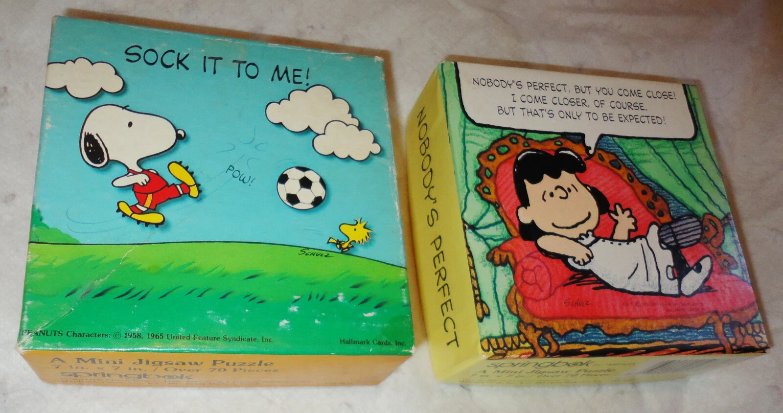
| 3.1.1 | 2014-07-10 | Sock it to Me | [150][151][152][153] | [154] |
| 3.1.0 | 2014-04-10 | Spring Dance | [103] | [155] |
| 3.0.3 | 2014-03-06 | Warm Puppy | [156] | [157] |
| 3.0.2 | 2013-09-25 | Frisbee Sailing | [158] | [159] |
| 3.0.1 | 2013-05-16 | Good Sport | [160] | [161] |
| 3.0.0 | 2013-04-03 | Masked Marvel | [162] | [163] |
| 2.15.3 | 2013-03-01 | Security Blanket | [164] | [165] |
| 2.15.2 | 2012-10-26 | Trick or Treat | [166] | [167] |
| 2.15.1 | 2012-06-22 | Roasted Marshmallows | [168] | [169] |
| 2.15.0 | 2012-03-30 | Easter Beagle | [170] | [171] |
| 2.14.2 | 2012-02-29 | Gift-Getting Season | See It's the Easter Beagle, Charlie Brown[172] | [173] |
| 2.14.1 | 2011-12-22 | December Snowflakes | [174] | [175] |
| 2.14.0 | 2011-10-31 | Great Pumpkin | See It's the Great Pumpkin, Charlie Brown[176] | [177] |
| r-devel | N/A | Unsuffered Consequences | [178] | [42] |
Interfaces
[edit]Examples of user interfaces for R
-
 Screenshot of the RKWard front-end running on the KDE 4 environment
 -
 R running in the emacs editor with the ESS package
 -


.png)
R is installed with a command line console by default, but there are multiple ways to interface with the language:
- Integrated development environment (IDE):
- R.app[179] (OSX/macOS only)
- Rattle GUI
- R Commander
- RKWard
- RStudio
- Tinn-R[180]
- General-purpose IDEs:
- Eclipse via the StatET plugin
- Visual Studio via R Tools for Visual Studio.
- Source-code editors:
- Other scripting languages:
- Python (website)
- Perl (website)
- Ruby (source code)
- F# (website)
- Julia (source code).
- General-purpose programming languages:
- Java via the Rserve socket server
- .NET C# (website)
Statistical frameworks that use R in the background include Jamovi and JASP.[citation needed]
Implementations
[edit]The main R implementation is written primarily in C, Fortran, and R itself. Other implementations include the following:
- pretty quick R (pqR), by Radford M. Neal, which attempts to improve memory management.
- Renjin for the Java Virtual Machine.
- CXXR and Riposte[181] written in C++.
- Oracle's FastR built on GraalVM.
- TIBCO Enterprise Runtime for R (TERR) to integrate with Spotfire.[182] (The company also created S-Plus, an implementation of the S language.)
Microsoft R Open (MRO) was an R implementation. As of 30 June 2021, Microsoft began to phase out MRO in favor of the CRAN distribution.[183]
Commercial support
[edit]
Although R is an open-source project, some companies provide commercial support:
- Oracle provides commercial support for its Big Data Appliance, which integrates R into its other products.
- IBM provides commercial support for execution of R within Hadoop.
See also
[edit]- Comparison of numerical-analysis software
- Comparison of statistical packages
- List of numerical-analysis software
- List of statistical software
- Rmetrics
Notes
[edit]- ^ This code displays to standard error a listing of all the packages that the tidyverse collection depends upon. The code may also display warnings showing namespace conflicts, which may typically be ignored.
- ^ Information about conferences and meetings is available in a community-maintained list on GitHub, jumpingrivers
.github .io /meetingsR / - ^ An expanded list of standard language features can be found in the manual "An Introduction to R", cran
.r-project .org /doc /manuals /R-intro .pdf
References
[edit]- ^ a b c Morandat, Frances; Hill, Brandon; Osvald, Leo; Vitek, Jan (11 June 2012). "Evaluating the design of the R language: objects and functions for data analysis". European Conference on Object-Oriented Programming. 2012: 104–131. doi:10.1007/978-3-642-31057-7_6. Retrieved 17 May 2016 – via SpringerLink.
- ^ Peter Dalgaard (13 June 2025). "R 4.5.1 is released". Retrieved 14 June 2025.
- ^ a b "R - Free Software Directory". directory.fsf.org. Retrieved 26 January 2024.
- ^ "R scripts". mercury.webster.edu. Retrieved 17 July 2021.
- ^ "R Data Format Family (.rdata, .rda)". Loc.gov. 9 June 2017. Retrieved 17 July 2021.
- ^ a b Hornik, Kurt; The R Core Team (12 April 2022). "R FAQ". The Comprehensive R Archive Network. 3.3 What are the differences between R and S?. Archived from the original on 28 December 2022. Retrieved 27 December 2022.
- ^ "Introduction". The Julia Manual. Archived from the original on 20 June 2018. Retrieved 5 August 2018.
- ^ "Comparison with R". pandas Getting started. Retrieved 15 July 2024.
- ^ Giorgi, Federico M.; Ceraolo, Carmine; Mercatelli, Daniele (27 April 2022). "The R Language: An Engine for Bioinformatics and Data Science". Life. 12 (5): 648. Bibcode:2022Life...12..648G. doi:10.3390/life12050648. PMC 9148156. PMID 35629316.
- ^ "Home - RDocumentation". www.rdocumentation.org. Retrieved 13 June 2025.
- ^ "R: What is R?". www.r-project.org. Retrieved 10 May 2025.
- ^ Ihaka, Ross. "The R Project: A Brief History and Thoughts About the Future" (PDF). p. 12. Archived (PDF) from the original on 28 December 2022. Retrieved 27 December 2022.
We set a goal of developing enough of a language to teach introductory statistics courses at Auckland.
- ^ Hornik, Kurt; The R Core Team (12 April 2022). "R FAQ". The Comprehensive R Archive Network. 2.13 What is the R Foundation?. Archived from the original on 28 December 2022. Retrieved 28 December 2022.
- ^ "Index of /datasets". lib.stat.cmu.edu. Retrieved 5 September 2024.
- ^ Ihaka, Ross. "R: Past and Future History" (PDF). p. 4. Archived (PDF) from the original on 28 December 2022. Retrieved 28 December 2022.
- ^ Ihaka, Ross (5 December 1997). "New R Version for Unix". stat.ethz.ch. Archived from the original on 12 February 2023. Retrieved 12 February 2023.
- ^ Ihaka, Ross. "The R Project: A Brief History and Thoughts About the Future" (PDF). p. 18. Archived (PDF) from the original on 28 December 2022. Retrieved 27 December 2022.
- ^ Wickham, Hadley; Cetinkaya-Rundel, Mine; Grolemund, Garrett (2023). R for Data Science, Second Edition. O'Reilly. p. xvii. ISBN 978-1-492-09740-2.
- ^ "Quarto". Quarto. Retrieved 5 September 2024.
- ^ Chambers, John M. (2020). "S, R, and Data Science". The R Journal. 12 (1): 462–476. doi:10.32614/RJ-2020-028. ISSN 2073-4859.
The R language and related software play a major role in computing for data science. ... R packages provide tools for a wide range of purposes and users.
- ^ Davies, Tilman M. (2016). "Installing R and Contributed Packages". The Book of R: A First Course in Programming and Statistics. San Francisco, California: No Starch Press. p. 739. ISBN 9781593276515.
- ^ Wickham, Hadley (2014). "Tidy Data" (PDF). Journal of Statistical Software. 59 (10). doi:10.18637/jss.v059.i10.
- ^ a b Wickham, Hadley; Cetinkaya-Rundel, Mine; Grolemund, Garrett (2023). R for Data Science, Second Edition. O'Reilly. ISBN 978-1-492-09740-2.
- ^ a b Hornik, Kurt (2012). "The Comprehensive R Archive Network". WIREs Computational Statistics. 4 (4): 394–398. doi:10.1002/wics.1212. ISSN 1939-5108. S2CID 62231320.
- ^ Kurt Hornik (23 April 1997). "Announce: CRAN". r-help. Wikidata Q101068595..
- ^ "The Status of CRAN Mirrors". cran.r-project.org. Retrieved 16 October 2024.
- ^ "CRAN - Contributed Packages". cran.r-project.org. Retrieved 16 October 2024.
- ^ "R-Forge: Welcome". r-forge.r-project.org. Retrieved 5 September 2024.
- ^ "The Omega Project for Statistical Computing". www.omegahat.net. Retrieved 5 September 2024.
- ^ "Build software better, together". GitHub. Retrieved 5 September 2024.
- ^ Wickham, Hadley; Grolemund, Garrett (January 2017). 1 Introduction | R for Data Science (1st ed.). O'Reilly Media. ISBN 978-1491910399.
{{cite book}}: CS1 maint: date and year (link) - ^ R Development Core Team. "Assignments with the = Operator". Retrieved 11 September 2018.
- ^ Kabacoff, Robert (2012). "Quick-R: User-Defined Functions". statmethods.net. Retrieved 28 September 2018.
- ^ Wickham, Hadley. "Advanced R - Functional programming - Closures". adv-r.had.co.nz.
- ^ "NEWS". r-project.org.
- ^ "R: R News". cran.r-project.org. Retrieved 14 March 2024.
- ^ Wickham, Hadley; Çetinkaya-Rundel, Mine; Grolemund, Garrett (2023). "4 Workflow: code style". R for data science: import, tidy, transform, visualize, and model data (2nd ed.). Beijing; Sebastopol, CA: O'Reilly. ISBN 978-1-4920-9740-2. OCLC 1390607935.
- ^ "Class Methods". Retrieved 25 April 2024.
- ^ Monkman, Martin. Chapter 5 R Release Names | Data Science with R: A Resource Compendium.
- ^ McGowan, Lucy D’Agostino (28 September 2017). "R release names". livefreeordichotomize.com. Retrieved 7 April 2024.
- ^ r-hub/rversions, The R-hub project of the R Consortium, 29 February 2024, retrieved 7 April 2024
- ^ a b c d Dalgaard, Peter (15 July 2018). "What's in a name? 20 years of R release management" (video). YouTube. Retrieved 9 April 2024.
- ^ "Read Peanuts by Charles Schulz on GoComics". www.gocomics.com. Retrieved 13 June 2025.
- ^ "[Rd] R 4.5.1 is released". hypatia.math.ethz.ch. Retrieved 13 June 2025.
- ^ "Read Peanuts by Charles Schulz on GoComics". www.gocomics.com. Retrieved 17 April 2025.
- ^ "[Rd] R 4.5.0 is released". hypatia.math.ethz.ch. Retrieved 17 April 2025.
- ^ "Read Peanuts by Charles Schulz on GoComics". www.gocomics.com. Retrieved 17 April 2025.
- ^ "[Rd] R 4.4.3 is released". hypatia.math.ethz.ch. Retrieved 17 April 2025.
- ^ Schulz, Charles (15 November 1957). "Peanuts by Charles Schulz for November 15, 1957 | GoComics.com". GoComics. Retrieved 6 January 2025.
- ^ "[Rd] R 4.4.2 is released". stat.ethz.ch. Retrieved 26 December 2024.
- ^ "Race for Your Life, Charlie Brown". IMDB. 3 August 1977. Retrieved 18 June 2024.
- ^ "R 4.4.1 is released". stat.ethz.ch. Retrieved 18 June 2024.
- ^ Schulz, Charles (29 June 1980). "Peanuts by Charles Schulz for June 29, 1980 | GoComics.com". GoComics. Retrieved 24 April 2024.
- ^ "R 4.4.0 is released". stat.ethz.ch. Retrieved 24 April 2024.
- ^ Schulz, Charles (29 June 1980). "Peanuts by Charles Schulz for June 29, 1980 | GoComics.com". GoComics. Retrieved 9 April 2024.
- ^ "R 4.3.3 is released". hypatia.math.ethz.ch. Retrieved 7 April 2024.
- ^ Schulz, Charles (31 October 1996). "Peanuts by Charles Schulz for October 31, 1996 | GoComics.com". GoComics. Retrieved 9 April 2024.
- ^ "[Rd] R 4.3.2 is released". stat.ethz.ch. Retrieved 7 April 2024.
- ^ Schulz, Charles (28 April 1979). "Peanuts by Charles Schulz for April 28, 1979 | GoComics.com". GoComics. Retrieved 9 April 2024.
- ^ "[Rd] R 4.3.1 is released". stat.ethz.ch. Retrieved 7 April 2024.
- ^ Schulz, Charles (13 June 1980). "Peanuts by Charles Schulz for June 13, 1980 | GoComics.com". GoComics. Retrieved 9 April 2024.
- ^ Schulz, Charles (16 June 1980). "Peanuts by Charles Schulz for June 16, 1980 | GoComics.com". GoComics. Retrieved 9 April 2024.
- ^ Schulz, Charles (26 November 1964). "Peanuts by Charles Schulz for November 26, 1964 | GoComics.com". GoComics. Retrieved 9 April 2024.
- ^ "[Rd] R 4.3.0 is released". stat.ethz.ch. Retrieved 7 April 2024.
- ^ Schulz, Charles (30 March 2001). "Peanuts by Charles Schulz for March 30, 2001 | GoComics.com". GoComics. Retrieved 9 April 2024.
- ^ "[Rd] R 4.2.3 is released". stat.ethz.ch. Retrieved 7 April 2024.
- ^ Schulz, Charles (30 October 1962). "Peanuts by Charles Schulz for October 30, 1962 | GoComics.com". GoComics. Retrieved 9 April 2024.
- ^ "[Rd] R 4.2.2 is released". stat.ethz.ch. Retrieved 7 April 2024.
- ^ Schulz, Charles (22 November 1970). "Peanuts by Charles Schulz for November 22, 1970 | GoComics.com". GoComics. Retrieved 9 April 2024.
- ^ Schulz, Charles (29 July 1971). "Peanuts by Charles Schulz for July 29, 1971 | GoComics.com". GoComics. Retrieved 9 April 2024.
- ^ Schulz, Charles (25 September 1969). "Peanuts by Charles Schulz for September 25, 1969 | GoComics.com". GoComics. Retrieved 9 April 2024.
- ^ Schulz, Charles (13 October 1973). "Peanuts by Charles Schulz for October 13, 1973 | GoComics.com". GoComics. Retrieved 9 April 2024.
- ^ Schulz, Charles (8 February 1974). "Peanuts by Charles Schulz for February 08, 1974 | GoComics.com". GoComics. Retrieved 9 April 2024.
- ^ Schulz, Charles (8 January 1970). "Peanuts by Charles Schulz for January 08, 1970 | GoComics.com". GoComics. Retrieved 9 April 2024.
- ^ "[Rd] R 4.2.1 is released". stat.ethz.ch. Retrieved 7 April 2024.
- ^ a b Schulz, Charles (6 March 1967). "Peanuts by Charles Schulz for March 06, 1967 | GoComics.com". GoComics. Retrieved 9 April 2024.
- ^ "[Rd] R 4.2.0 is released". stat.ethz.ch. Retrieved 7 April 2024.
- ^ a b "[Rd] R 4.1.2 is released". hypatia.math.ethz.ch. Retrieved 7 April 2024.
- ^ Schulz, Charles (1 November 1967). "Peanuts by Charles Schulz for November 01, 1967 | GoComics.com". GoComics. Retrieved 9 April 2024.
- ^ Schulz, Charles (12 July 1967). "Peanuts by Charles Schulz for July 12, 1967 | GoComics.com". GoComics. Retrieved 9 April 2024.
- ^ Schulz, Charles (17 May 1978). "Peanuts by Charles Schulz for May 17, 1978 | GoComics.com". GoComics. Retrieved 9 April 2024.
- ^ "[Rd] R 4.1.1 is released". hypatia.math.ethz.ch. Retrieved 7 April 2024.
- ^ Schulz, Charles (12 February 1986). "Peanuts by Charles Schulz for February 12, 1986 | GoComics.com". GoComics. Retrieved 8 April 2024.
- ^ "[Rd] R 4.1.0 is released". hypatia.math.ethz.ch. Retrieved 7 April 2024.
- ^ Schulz, Charles (30 July 1978). "Peanuts by Charles Schulz for July 30, 1978 | GoComics.com". GoComics. Retrieved 7 April 2024.
- ^ "[Rd] R 4.0.5 is released". hypatia.math.ethz.ch. Retrieved 7 April 2024.
- ^ Schulz, Charles (2 March 1959). "Peanuts by Charles Schulz for March 02, 1959 | GoComics.com". GoComics. Retrieved 7 April 2024.
- ^ Schulz, Charles (27 February 2006). "Peanuts by Charles Schulz for February 27, 2006 | GoComics.com". GoComics. Retrieved 7 April 2024.
- ^ Schulz, Charles (13 March 1959). "Peanuts by Charles Schulz for March 13, 1959 | GoComics.com". GoComics. Retrieved 7 April 2024.
- ^ "[Rd] R 4.0.4 scheduled for February 15". hypatia.math.ethz.ch. Retrieved 7 April 2024.
- ^ Schulz, Charles (23 October 1972). "Peanuts by Charles Schulz for October 23, 1972 | GoComics.com". GoComics. Retrieved 7 April 2024.
- ^ "[Rd] R 4.0.3 is released". stat.ethz.ch. Retrieved 7 April 2024.
- ^ Schulz, Charles (14 April 1962). "Peanuts by Charles Schulz for April 14, 1962 | GoComics.com". GoComics. Retrieved 7 April 2024.
- ^ "R 4.0.2 is released". hypatia.math.ethz.ch. Retrieved 7 April 2024.
- ^ Schulz, Charles (6 February 1962). "Peanuts by Charles Schulz for February 06, 1962 | GoComics.com". GoComics. Retrieved 7 April 2024.
- ^ "R 4.0.1 is released". hypatia.math.ethz.ch. Retrieved 7 April 2024.
- ^ Schulz, Charles (24 April 1970). "Peanuts by Charles Schulz for April 24, 1970 | GoComics.com". GoComics. Retrieved 7 April 2024.
- ^ "R 4.0.0 is released". hypatia.math.ethz.ch. Retrieved 7 April 2024.
- ^ Schulz, Charles (29 February 2000). "Peanuts by Charles Schulz for February 29, 2000 | GoComics.com". GoComics. Retrieved 7 April 2024.
- ^ "R 3.6.3 is released". hypatia.math.ethz.ch. Retrieved 7 April 2024.
- ^ Schulz, Charles (12 July 1965). "Peanuts by Charles Schulz for July 12, 1965 | GoComics.com". GoComics. Retrieved 7 April 2024.
- ^ "R 3.6.2 is released". hypatia.math.ethz.ch. Retrieved 7 April 2024.
- ^ a b Schulz, Charles (22 March 1971). "Peanuts by Charles Schulz for March 22, 1971 | GoComics.com". GoComics. Retrieved 7 April 2024.
- ^ "R 3.6.1 is released". hypatia.math.ethz.ch. Retrieved 7 April 2024.
- ^ Schulz, Charles (3 March 1963). "Peanuts by Charles Schulz for March 03, 1963 | GoComics.com". GoComics. Retrieved 7 April 2024.
- ^ "R 3.6.0 is released". hypatia.math.ethz.ch. Retrieved 7 April 2024.
- ^ Schulz, Charles (11 March 1959). "Peanuts by Charles Schulz for March 11, 1959 | GoComics.com". GoComics. Retrieved 7 April 2024.
- ^ "R 3.5.3 is released". stat.ethz.ch. Retrieved 7 April 2024.
- ^ Schulz, Charles (25 January 1960). "Peanuts by Charles Schulz for January 25, 1960 | GoComics.com". GoComics. Retrieved 7 April 2024.
- ^ "R 3.5.2 is released". stat.ethz.ch. Retrieved 7 April 2024.
- ^ Schulz, Charles (9 March 1972). "Peanuts by Charles Schulz for March 09, 1972 | GoComics.com". GoComics. Retrieved 7 April 2024.
- ^ "R 3.5.1 is released". stat.ethz.ch. Retrieved 7 April 2024.
- ^ Schulz, Charles (27 January 1973). "Peanuts by Charles Schulz for January 27, 1973 | GoComics.com". GoComics. Retrieved 7 April 2024.
- ^ "R 3.5.0 is released". hypatia.math.ethz.ch. Retrieved 7 April 2024.
- ^ "It's nice to have a friend you can lean on". Archived from the original on 7 April 2024.
- ^ "Peanuts Snoopy Charlie Brown A Friend is Someone you can lean on metal tin sign". Retrieved 17 April 2025.
- ^ "Peanuts Snoopy & Charlie Brown Friend Is Someone You Can Lean On Fire-King Mug". Retrieved 17 April 2025.
- ^ "R 3.4.4 is released". hypatia.math.ethz.ch. Retrieved 7 April 2024.
- ^ Schulz, Charles (19 February 1967). "Peanuts by Charles Schulz for February 19, 1967 | GoComics.com". GoComics. Retrieved 7 April 2024.
- ^ "R 3.4.3 is released". hypatia.math.ethz.ch. Retrieved 7 April 2024.
- ^ "R 3.4.2 is released". hypatia.math.ethz.ch. Retrieved 7 April 2024.
- ^ a b Schulz, Charles (9 September 1965). "Peanuts by Charles Schulz for September 09, 1965 | GoComics.com". GoComics. Retrieved 7 April 2024.
- ^ "R 3.4.1 is released". hypatia.math.ethz.ch. Retrieved 7 April 2024.
- ^ "R 3.4.0 is released". stat.ethz.ch. Retrieved 7 April 2024.
- ^ Schulz, Charles (29 June 1966). "Peanuts by Charles Schulz for June 29, 1966 | GoComics.com". GoComics. Retrieved 7 April 2024.
- ^ "[R] R 3.3.3 is released". stat.ethz.ch. Retrieved 7 April 2024.
- ^ Schulz, Charles (30 October 1968). "Peanuts by Charles Schulz for October 30, 1968 | GoComics.com". GoComics. Retrieved 7 April 2024.
- ^ "[R] R 3.3.2 is released". stat.ethz.ch. Retrieved 7 April 2024.
- ^ Schulz, Charles (15 June 1967). "Peanuts by Charles Schulz for June 15, 1967 | GoComics.com". GoComics. Retrieved 7 April 2024.
- ^ "[R] R 3.3.1 is released". stat.ethz.ch. Retrieved 7 April 2024.
- ^ Schulz, Charles (7 May 1971). "Peanuts by Charles Schulz for May 07, 1971 | GoComics.com". GoComics. Retrieved 7 April 2024.
- ^ "[R] R 3.3.0 is released". stat.ethz.ch. Retrieved 7 April 2024.
- ^ a b Schulz, Charles (20 February 1964). "Peanuts by Charles Schulz for February 20, 1964 | GoComics.com". GoComics. Retrieved 7 April 2024.
- ^ "VERSION-NICK". Retrieved 7 April 2024.
- ^ "R 3.2.5 is released". stat.ethz.ch. Retrieved 7 April 2024.
- ^ "R 3.2.4-revised is released". stat.ethz.ch. Retrieved 7 April 2024.
- ^ "R 3.2.4 is released". stat.ethz.ch. Retrieved 7 April 2024.
- ^ Schulz, Charles (18 December 1980). "Peanuts by Charles Schulz for December 18, 1980 | GoComics.com". GoComics. Retrieved 9 April 2024.
- ^ "R 3.2.3 is released". stat.ethz.ch. Retrieved 7 April 2024.
- ^ MarketScreener (7 October 2008). "METLIFE : Brush Up on Fire Safety Basics -October 07, 2008 at 04:03 pm EDT | MarketScreener". www.marketscreener.com. Retrieved 7 April 2024.
- ^ "MetLife Advises People to Brush Up on Fire Safety Basics to Stay Safe". Claims Journal. 12 October 2005. Retrieved 7 April 2024.
- ^ "R 3.2.2 is released". stat.ethz.ch. Retrieved 7 April 2024.
- ^ Schulz, Charles (10 March 1969). "Peanuts by Charles Schulz for March 10, 1969 | GoComics.com". GoComics. Retrieved 7 April 2024.
- ^ "[R] R 3.2.1 liftoff". stat.ethz.ch. Retrieved 7 April 2024.
- ^ Schulz, Charles (7 April 1966). "Peanuts by Charles Schulz for April 07, 1966 | GoComics.com". GoComics. Retrieved 7 April 2024.
- ^ "[R] R 3.2.0 is released". stat.ethz.ch. Retrieved 7 April 2024.
- ^ Schulz, Charles M. (2019). Happiness is a warm puppy. New York : Penguin Workshop. ISBN 978-1-5247-8995-4.
{{cite book}}: CS1 maint: publisher location (link) - ^ "R 3.1.3 is released". stat.ethz.ch. Retrieved 7 April 2024.
- ^ "[R] R 3.1.2 is released". stat.ethz.ch. Retrieved 7 April 2024.
- ^ "Sock it to me". Archived from the original on 9 April 2024.
- ^ "Sock it to me". Archived from the original on 9 April 2024.
- ^ "Sock it to me puzzle". Archived from the original on 9 April 2024.
- ^ "Peanuts Springbok Puzzles".
- ^ "[R] R 3.1.1 is released". stat.ethz.ch. Retrieved 7 April 2024.
- ^ "[R] R 3.1.0 is released". stat.ethz.ch. Retrieved 7 April 2024.
- ^ Schulz, Charles (11 January 1965). "Peanuts by Charles Schulz for January 11, 1965 | GoComics.com". GoComics. Retrieved 7 April 2024.
- ^ "R 3.0.3 is released". stat.ethz.ch. Retrieved 7 April 2024.
- ^ Schulz, Charles (3 September 1971). "Peanuts by Charles Schulz for September 03, 1971 | GoComics.com". GoComics. Retrieved 7 April 2024.
- ^ "R 3.0.2 is released". stat.ethz.ch. Retrieved 7 April 2024.
- ^ Schulz, Charles (22 November 1953). "Peanuts by Charles Schulz for November 22, 1953 | GoComics.com". GoComics. Retrieved 7 April 2024.
- ^ "R 3.0.1 is released". stat.ethz.ch. Retrieved 7 April 2024.
- ^ Schulz, Charles (23 June 1981). "Peanuts by Charles Schulz for June 23, 1981 | GoComics.com". GoComics. Retrieved 7 April 2024.
- ^ "R 3.0.0 is released". stat.ethz.ch. Retrieved 7 April 2024.
- ^ Schulz, Charles (23 October 1965). "Peanuts by Charles Schulz for October 23, 1965 | GoComics.com". GoComics. Retrieved 7 April 2024.
- ^ "R 2.15.3 is released". stat.ethz.ch. Retrieved 7 April 2024.
- ^ Schulz, Charles (31 October 1969). "Peanuts by Charles Schulz for October 31, 1969 | GoComics.com". GoComics. Retrieved 7 April 2024.
- ^ "R 2.15.2 is released". stat.ethz.ch. Retrieved 7 April 2024.
- ^ Schulz, Charles (6 June 1987). "Peanuts by Charles Schulz for June 06, 1987 | GoComics.com". GoComics. Retrieved 7 April 2024.
- ^ "R 2.15.1 is released". stat.ethz.ch. Retrieved 7 April 2024.
- ^ Schulz, Charles (11 April 1971). "Peanuts by Charles Schulz for April 11, 1971 | GoComics.com". GoComics. Retrieved 7 April 2024.
- ^ "R 2.15.0 is released". stat.ethz.ch. Retrieved 7 April 2024.
- ^ It's the Easter Beagle, Charlie Brown! (TV Short 1974) - Quotes - IMDb. Retrieved 8 April 2024 – via www.imdb.com.
- ^ "R 2.14.2 is released + R anniversary". stat.ethz.ch. Retrieved 7 April 2024.
- ^ McGough, Nellah Bailey (20 January 2023). "Our Favorite Quotes and Sayings from "A Charlie Brown Christmas"". Southern Living. Retrieved 8 April 2024.
- ^ "R 2.14.1 is released". stat.ethz.ch. Retrieved 7 April 2024.
- ^ Schulz, Charles (29 October 1973). "Peanuts by Charles Schulz for October 29, 1973 | GoComics.com". GoComics. Retrieved 7 April 2024.
- ^ "R 2.14.0 is released". stat.ethz.ch. Retrieved 7 April 2024.
- ^ Schulz, Charles (17 August 1967). "Peanuts by Charles Schulz for August 17, 1967 | GoComics.com". GoComics. Retrieved 7 April 2024.
- ^ "R for macOS". cran.r-project.org. Retrieved 5 September 2024.
- ^ "IDE/Editor para Linguagem R | Tinn-R - Home". Tinn-R (in Brazilian Portuguese). Retrieved 5 September 2024.
- ^ Talbot, Justin; DeVito, Zachary; Hanrahan, Pat (1 January 2012). "Riposte: A trace-driven compiler and parallel VM for vector code in R". Proceedings of the 21st international conference on Parallel architectures and compilation techniques. ACM. pp. 43–52. doi:10.1145/2370816.2370825. ISBN 9781450311823. S2CID 1989369.
- ^ Jackson, Joab (16 May 2013). TIBCO offers free R to the enterprise. PC World. Retrieved 20 July 2015.
- ^ "Looking to the future for R in Azure SQL and SQL Server". 30 June 2021. Retrieved 7 November 2021.
Further reading
[edit]- Wickham, Hadley; Çetinkaya-Rundel, Mine; Grolemund, Garrett (2023). R for data science: import, tidy, transform, visualize, and model data (2nd ed.). Beijing Boston Farnham Sebastopol Tokyo: O'Reilly. ISBN 978-1-4920-9740-2.
- Gagolewski, Marek (2024). Deep R Programming. doi:10.5281/ZENODO.7490464. ISBN 978-0-6455719-2-9.
External links
[edit]- R Technical Papers
- Big Book of R, curated list of R-related programming books
- Books Related to R - R Project, partially annotated curated list of books relating to R or S.
| Features | ||
|---|---|---|
| Implementations |
| |
| Packages | ||
| Interfaces | ||
| People | ||
| Organisations |
| |
| Publications | ||
| International | |
|---|---|
| National | |
| Other | |